Game stopping bug with Topspin…

I’ve encountered a bug with Topspin on Windows 10, which gives a blue-screen of death. I responded to a users call for help, and after some fiddling; fixed/worked around the problem.

I believe it related to processing data on a cloud drive; in this case it was Microsoft’s own One drive.  Once the processing was changed to a local folder; with no cloud synchronisation ‘features’, the problem went away.

Its possible this behaviour is also to be found with OS X. I had another report of a user saying ‘Topspin doesn’t work and gives weird and funny messages and I had to restart the computer…’ I didn’t have time to investigate, other than to try processing on a non-syncing folder; which worked.

I’d also like to point out that storing processed data generally may not be what you want to do, for routine work at least. It can become vast, and if you store all your data indiscriminately ; you’ll rapidly chew through storage space and network bandwidth if you cloud-sync it. (I processed a ‘Perfect-clip-hsqc’ recently to a high resolution. You could resolve carbons 1.5Hz apart quite easily; but the data was 17.2Gb in size…)

 

Apple OS X Mojave and Topspin

It works!

At least so far I haven’t found any show-stopping bugs after about a week on my system.

 

Mid-2015 15″ MacBook Pro

Mojave 10.14 Beta (18A384a) (I think that’s user beta 9, installed 2018-09-07)

Topspin 4.0.5

 

As ever, your milage may vary… On mission critical systems; take a Time Machine backup first. Make sure the backup works! Consider backing up the backup; as this is now your only *known* working version.

Note. I installed Mojave as an upgrade to High Sierra and *after* I had installed Topspin.

 

High-resolution screens and Topspin.

Have you had trouble using Topspin with a high resolution 4K screen? Well; trouble no more! Probably. Bruker have released version 4.0.3 of Topspin; which gives you the option to choose between some default configurations of icons/font size to better match different monitor resolutions.

Choose ‘All in One Fonts and Icon Size’ from the preferences, click ‘save’ and then ‘Apply’ from the preferences windows and restart Topspin.

I don’t actually have a high resolution screen to test it out with however! But that didn’t stop me fiddling with it anyway…

Now this didn’t work for me initially on my Macbook Air… Previously I’d spent a long time tampering with the settings to get something viewable via a projector in a lecture theater. Initially changing the options seemed to have little effect. After choosing ‘Reset…’ from the preference menu; the options did change things; however the fonts didn’t look to have the correct weight for the size option. It was only by deleting the hidden .topspin1 directory from my home directory I was able to get it to behave how I was expecting it to.

Note, the reset/deleting the folder will put Topspin back to it default appearance, and you’ll loose any customisation to its appearance/default directories in the databrowser.

 

 

Topspin and VirtualBox

It is possible to run Topspin within VirtualBox quite easily. On my late 2013 MacBook Air I’ve installed version 4 into virtual Windows 8.1 and linux CentOs 7 and it works very nicely. In fact the CentOs version seems to do NUS processing very well; at near native speeds.

There is however some tips I’m going to pass on about management of the virtual hard disk of the Windows8.1 guest.

When I set the virtual machine up I choose to have a 128 GB dynamic disk thinking ‘that’ll be alright; probably the windows install won’t take up more than 20 GB’ And I was right; however in the years I’ve been using it; the size of the VDI file on my Mac grew to about 64GB.

My advice is; when you set up the virtual machine and install windows DON’T make the system partition fill the maximum size of the dynamically allocated space you made. Make a partition about 30 GB in size.

Here’s my little journey over the two days it took me to sort it out.

I went through update after update until there were no more updates. I hadn’t booted the virtual Windows machine for about 3 months; so this too some time.

After cleaning the temporary files (type ‘disk clean’ into the search box); going through all the options, including deleting windows update files, I got windows to report it was using about 23GB. However the size of the VDI file on my Mac remained the same.

This is a known feature of dynamic disks and the way files are deleted in the guest; deletion still leaves the information on the disk; it just removes the information on how to access it. So the VirtualBox manager has know way of knowing whats a ‘real’ file and a deleted one.

There is a command that will compact a VDI file; the algorithm it uses is (probably) :-

Scan to the last used cluster of the disk; if all the subsequent sectors have zero in them; compact the disk to the last used cluster.

The problem with Windows is that as you use it; it will scatter information across a lot of the disk. So even if you use a utility to set all unused clusters to zero (which will include previously deleted files), you still may not be able to shrink the VDI file as much as you might like.

See ‘Shrink VirtualBox VDi’ for instructions on the above. Note I found the sdelete command didn’t work the way I hoped… As it ran the size on the VDI file grew until it filled my mac. So I used the below method instead…

So, in the ‘good old days’ you could defragment your disk and compact the free space; leaving the end of your disk clear. However, with modern SSD disks; defragging is frowned upon and in fact you can’t really do it in Windows. You can ‘optimise’ but this doesn’t seem to consolidate free space.

I had to download the free version of Auslogics Disk Defrag Pro to do a basic defrag; the free version doesn’t consolidate free space however. Sigh. It did help; after running it, the last used cluster was around the 40GB mark. And by clicking on the cluster I could see it was unmovable and in C:\SystemVolumeInformation See the information in the link on how to remove this file.

I then ran the defrag pro tool again. Most of the unmovable file was now gone; however one cluster remained near the end of the disk, which looked to be used by the filesystem management itself…. So. Next bit of fiddling…

I then used the ‘Administrative Tools=>Computer Management=>Storage=>Disk Management to shrink the C: disk to about 3GB above its minimum (23GB) size. Hurrah! It worked!

I know had a disk that I knew only contained files within a 26GB boundary! So, shutdown the virtual computer, go to an OX X command line and type :-

VBoxManage modifymedium –compact /path/to/thedisk.vdi

Blast. The virtual disk size is *still* 60GB. At this point if it were a Linux guest I’d be screaming ‘FSCKing FSCK!!!!‘ I knew I had a 26GB C: disk and about 98GB on unallocated space on the Windows virtual machine. So what gives? Those deleted files must still have not had zeros written to them.

Next. Boot up Windows again; allocate the free space to a new disk; quick format it; delete the disk again; shutdown; vboxmanage… Blast it! Still 60GB!

Boot up windows; untick the ‘quickformat’ option on the disk creation/format; delete the disk when done; shutdown; vboxmanage… Hurray! Finally a VDI disk 26GB in size and now I have 36GB free on my Mac!

So. To recap.

1. Make sure you’ve installed all the windows updates. You don’t want microsoft mucking it all up by writing stuff to your disk whilst fiddling about with it.
2. Delete everything you can. Type ‘disk clean’ into the search box in windows; go through all the options.
3. Defragment the drive as much as possible.
   1. Optional. Turn off the recovery options. Type ‘view advanced system settings’ into the search box, go to system protection and turn off the recovery options. Note you won’t be able to restore to an older (working) point if your windows installation goes wrong.
4. Shrink the partition to a few GB larger than the reported used amount on the disk. Type ‘administrative tools’ into the search and choose computer management=>storage=>disk management and shrink volume.
5. Format the remaining free space; making sure you’ve unchecked the quick format box. Delete the partition again.
6. Use the VBoxManage modifymedium –compact /path/to/thedisk.vdi to shrink the VDI file.

If you need more space in Windows; you can use the management tools to gradually increase the size of the partition.

A short cut to dimension N

Faster or better? Faster and better?

Multi-dimensional NMR is incredibly powerful, and often for all but the simplest problems; essential for structural elucidation. Sure you can spend time planning, running and interpreting a lot of different 1D experiments that could solve your problem; but often typing a few commands can give you a 2D spectrum that shows you at a glance what you need to see.

Its just a shame it takes so long… A 2D result typically consists of 256 1D experiments; each with x number of scans. If you need to increase the signal to noise; or increase the resolution (in the derived dimensions), the length of time it takes goes up geometrically; its even worse the higher number of dimensions you need to use…

But thinking about just a 2D experiment; if you look at it; its mostly empty space. Really the information you get out of it is list of peaks, described by two frequencies… Surely there ought to be a way to ‘compress’ this at the acquisition level?

Turns out there is; using several different methods. As to how they work; well much the same way as the ‘inertial dampeners’ do on the Star Ship Enterprise; which is to say ‘very well’ I really don’t have the mathematical capability to do a proper explanation. Best I can do is analogies… Which can only go so far, and may actually contravene the laws of physics!

Non-Uniform Sampling.

I asked the question in an early post ‘How many points do you need to represent a sine wave?’ Turns out, not so many… The way this ‘NUS’ technique works is to only sample some of the points in the derived dimensions. For a 2D spectrum; maybe around 25%, for a 3D maybe around 5%; this gives a huge speed up. You then use signal processing techniques to recover the missing points.

So what you do is prepare a ‘sparse sample schedule’ which contains a list of the slices; that is the 1D spectra with the corresponding delays from the full 2D. Ordinarily; you setup your 256 increment HSQC and you get 256 1D spectra each run with equally incremented delays. Using NUS, you might get 32 1D spectra; each run with non-equally incremented delays.

This method works very well for experiments such as HSQC where you tend to only have one peak at a given frequency in F2 (The carbon dimension); and less well for experiments such as COSY or HMBC where you have multiple peaks at a given F2 frequency. And I can’t really get very nice results at all with NOESY. I believe this is because you inherently need more points to represent the more complicated sine/cosine wave you’re trying to calculate to do the final FT on. The quality is also very dependent on the algorithm used for the reconstruction. The results I’ve obtained have all been processed with the same method using Brukers Topspin software. I’ve tried NMRpipe and MDDnmr; and I have some success with HSQC; but just haven’t had the time to put on the crampons and break out the ice-axe to go up the near vertical learning curve for NMRpipe.

Problems with going too quick.

You might think, ‘Thats amazing! I can run everything four times quicker!!!’

As with everything; you don’t get something for nothing…

So. Problems. If you sample at too low a level; you can find the frequencies of the peaks may shift slightly. Also you’ll get more noise in the spectrum. If you extract a row from the 2D you see this noise is ‘non-guassian’ and has the appearance of spikes scattered randomly through the spectrum.

Except it’s not random. It’s dependent on the sparse sample list you used; some schedules may be better than others for a given distribution of frequencies. I tried a list of prime numbers; gave a *very* poor result. Random points are better; random points with a Poisson distribution bias towards the start may be even better and help with poor s/n.

There’s a whole load of papers about schedule generation; but the upshot seems to be there’s no easy way to calculate the best schedule.  Also because you don’t necessarily know what peaks you’re going to see; there may be no general way to calculate the ‘best’ schedule.

If your s/n is inherently small; these artefacts can rapidly overwhelm your sample peaks. So sparse, non-uniform sampling may not be appropriate for very dilute samples. As they say, ‘your mileage may vary’.

I find that with simple organic compounds; running a 256 point HSQC at 25% for 2 scans per increment works well; this can be done in around 2 minutes. You might be able to to it in 1 minute; but I prefer being more certain it will work. For simple compounds, COSY I do at 37.5% of 256, 2 scans; HMBC, 37.5% of 360 and 2 scans. For more resolution I do COSY at 37.5% of 512, HSQC 25% of 1024 and HMBC at 37.5% of 768. You should look at your results critically though, if you’re missing peaks you might expect, further investigation may be required!

Enhance! Enhance!

So you might be able to to things faster; how about better? again, take an HSQC, our standard experiment is 256 increments over about 180ppm; this gives a resolution at 500 MHz of around 180Hz in F1. So the peaks quite often overlap in crowded areas. What can NUS do for this?

Turns out quite a lot.

Here’s a DEPT135 edited HSQC, 25% of 256 points. Took about 2mins 19 seconds. Looks perfectly good…

Here’s a zoom.

Here’s a zoom of 25% of 1024 points; took about 8mins 28 seconds. Looks good…

Lets enhance… 25% of 2048, took less than 17 mins.

Enhance! Enhance! 25% of 24K points! 3hrs 17 mins. A long time; but look at the resolution!

Faster! Faster! The s/n is good; lets do 3.125% of 24K points… Only takes 25 mins. You’ve got to look carefully to see a difference. Note the full 24K points would take 16hrs 37mins…

. I would say the 2D spectra of the 25% version looks slightly better though when you only scale to remove the noise. If you actually look carefully at the noise; the 3.125% (rd) is a lot worse… Its hard to quantify, as its non-Gaussian; but there’s a lot more spikes.

Here’s the calculated sum of both 24K spectra; to produce a calculated DEPT135. Not much noise in either of them

Zoom and enhance… You can resolve peaks about 3Hz apart.

Just to show the same region at 2048K and 256K, where we started.

So, with a nice sample you can run samples faster, even faster and with better resolution in some instances.

APSY

This is another method of speeding up multi-dimensional acquisition of 3 and above.

I think a good way to describe this is to imagine dropping some stones into a pool at the same time… The ripples spread outwards. Then imagine you freeze the surface before the waves hit the edges. If you then take slices through the surface at different angles; how many slices to you need to re-construct the positions of the stones?

I’ve never run any of these; so I can’t say much more about how well it works in practice. About as well as those inertial dampers I expect.

Here’s a reference.

https://www.ncbi.nlm.nih.gov/pubmed/21710379

Multi-dimensional NMR

Not going to go into much detail here; its incredibly versatile and powerful. You can find far better explanations elsewhere as to how it actually works; again I’d recommend James Keeler. Heres a video intro…

‘James Keeler – 2D NMR Part I’

Its advancing all the time; even some of the basic 2D techniques you’re used to are being developed and extended.

I’m going to note a few practical points about the acquisition, focusing on 2D NMR.

Intro

Your actual result is composed of a series of 1D results; each of which has something varied in it. The Bruker acquisition software ‘packages’ these into a single file called ‘ser’, regardless of the dimensionality of the experiment. It creates this file on the hard disk of the spectrometer before the experiment runs (filled with zeros) and copies each 1D result into it as the experiment runs.

Acquisition

So you can transform the result as the experiment progresses; this can be useful if you want to check if its going to work. What I quite often do is transform the spectrum after a few increments and extract one of the rows and transform that. So for a HSQC for instance the Bruker commands are :-

rser 2

sinm;fp

If you see no signals at all; you may need to run more scans per increment. If you see loads of signal then you may not need as many. 2D experiments appear to be quite sensitive as you throw away all the noise when you look at the result; so you really only need a little signal for the experiment to work. I’d recommend having a look at some of the data you have to get a feel for how long an acquisition might take; given the transform of a row at the start of the experiment.

Processing (2d)

The full 2d transform is done by typing ‘xfb’

Its worth having a look at the result of typing ‘xf2’ to transform just the rows. Here’s an example of doing that on an HSQC and zooming into a peak. You can probably see there’s some kind of function decaying away; which you could Fourier transform.

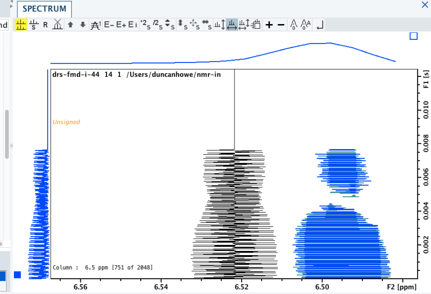It can be worth looking at the actual rows themselves, the 1d slices that the full experiment is made up of; as you may be able to identify experimental artefacts, which could affect the final result.

So for instance a problem with one of our probes gave phase errors; the inconsistencies with phase were readily apparent by looking at the 1d slices of a NOESY experiment. Problems with vibration will cause noise around peaks, which will be visible; this will translate into ‘T1 noise’ in the final spectrum.

You can play around with the window functions and the resolution, but that can be a bit of a black art… If you can see what you need its probably ok! We usually use as a starting point (for a 1.8K x 256 HSQC) :-

 

Temperature Calibration Revisited

Some further notes about accurate temperatures in NMR measurements.

I’ve spent ages running all kinds of experiments trying to work out the best way to calibrate temperatures. The upshot; you can get calibration curves that are very good; peaks fitting a function with an R-value of nearly 1; but all the calibration samples give different curves.

I was asked to run some cobalt spectra; it hadn’t been set up on the instrument; so in with the test sample. I noticed the lineshape wasn’t perfect, and knowing the chemical shift is dependent on temperature I thought I’d try a different temperature. Whilst the temperature was changing, I happened to run a spectrum. The line was sharper and became broader as equilibrium was reached! I coloured this in as ‘Interesting, probably convection currents mix the sample, sharpening the line’

And there I left it for some years; until I was asked to run some slice selective NMR experiments. After I had the method sorted (getting a pseudo 2D spectrum that’s a ‘map’ of the Z-axis of the sample) I revisited the cobalt sample. Here’s the result, which observes slices through the Z-axis of the sample.

 

And slice 15 (near the top of the tube where the gradient slackens off) with the conventional 1D spectrum overlaid.

The individual slices are symmetrical, and the sum of them looks like the conventional spectrum. So I put this down to a temperature gradient in the probe over the Z-axis. It could be a Z shim misalignment; a Z shim deviation may look exactly like a temperature gradient, but I doubt the Z-shims are far out…

For a bit of fun I’ve also run the slice selective experiment after deliberately misaligning the Z shims. You get a nice map of the relevant shim functions. (Heres Z1 through Z4, using the 1% CHCl3 in acetone line shape test sample.)

 

So, what you observe is an average of temperature over the volume of your sample, and any z-shim misalignment which *may* confound the temperature measurement further.

 

1D processing.

First a few principles and things to think about.

You commonly go from a FID (information which changes with time) to a spectrum (information that changes with frequency) by using the Fourier transform algorithm.

• An infinitely sharp line would take an infinitely long time to decay away.
• The Fourier transform of noise is noise.
• How many points do you need to calculate a sine function accurately?

You can disappear off down a lot of rabbit holes finding out about digitisation and signal processing; just google the ‘Nyquist theorem’ But if you just think about what you might need to capture to calculate a result…

If its a pure sine function (i.e. never decays or changes), not so many points, in principle you might be able to do it with two. If it decays; you’ll need more to calculate the decay function. If you have sine-waves over lapping and decaying, even more. If you have a lot of very sharp lines, all with very similar frequencies (as in a few Hz or less); you might need to acquire for a long time, digitising a lot of points, maybe 128,000 or more, as the frequencies will only start to diverge after the sine-waves have been through enough cycles.

A bit about acquisition.

The spectrum of your sample is of course dependent on physics. You can use the laws of physics to take the spectrum and infer physical values about your sample. (Going in the other direction, taking your molecule and using physics to infer your spectrum is tricky…) The best way to work out how to do this, is to work through James Keelers lectures; they’ll tell you pretty much everything you’ll need to know. I’d particularly recommend the relaxation chapters. The sharpness of your lines is going to depend on the ‘T2’ relaxation parameter; short T2 values give broad lines. The T1 parameter measures how long it takes the spins to return to equilibrium.

The information you need is typically frequencies and the amplitude of those frequencies. If you don’t digitise enough points over a long enough time; you may not be able to resolve all the frequencies. If you pulse too quickly, the spins may not have time to return to equilibrium and so the amplitude of the frequencies may not be accurate.

Some basic processing.

In a way this is basic ‘retouching’. The simplest way to improve the appearance is to apply an appropriate weighting function to your FID; which is to multiply each point by a certain value. Say if you have quite a broad signal, you can progressively attenuate the signal over time, which will remove the noise from it. This is the most common function; exponential multiplication, using positive values; also known as line broadening. Usually proton spectra look good with 0.1 – 0.3 Hz of LB; carbons might use 1Hz or more; but its dependent on what you what to see…

There are other functions you can use, which might improve linewidth (resolution), such as gaussian functions. In principle there’s no limit to what you could do.

Other tweaks :-

• Zero Filling. Increasing the digital resolution; if you have acquired points A and C from a sine wave; you can imagine you have a pretty good chance of  interpolating B.
• Fowards Prediction. If you’ve captured the first half of the decaying sine function, you’ve got a good chance of predicting the second half.
• Backwards Prediction. You can remove broad humps by zeroing the first part of the FID (very broad humps will only be represented by a few points at the start) and then calculating the zeroed part to compensate.

Case Studies

Getting some sharp lines.

So here’s an example where I had to go through pretty much all of the above… Resolution enhancement of a 13C spectrum. Theoretically carbon spectra can have very sharp lines; but usually the extra noise present (compared to 1H) and the fact the lines are usually quite far apart means that you use a few Hz of line broadening to make the spectra look nice. I ran this spectrum and noticed this region looked like there was additional structure hidden in the broad lines.

Decreasing the line broadening from 3 to 1 gave this.

Setting it to 0 gave this.

This shows the limits of what might be possible with the FID (64K, acquisition time of 1s) You can perhaps do a bit more; here’s linear prediction of the FID out to 256K. (memod=LPfc, NoCoef=4096, lb=0)

So, it actually seems that this spectrum requires more acquisition points. Cutting to the chase, here’s the result that approaches the limit of what is probably possible with this instrument.

From the stacked plots below, which show the actual data points of 64K, 128K, 256K, 512K and 1024K spectra, you might conclude 1024K points is probably overkill; 512K points looks good and 256K is probably enough for most purposes.

This is confirmed by doing forwards-prediction out to 1024K points. I’ve tried taking the 1024K spectra and enhancing it further with gaussian functions; but this looks as good as it gets.

However I’d make the point that you don’t know what other algorithms exist; or might exist in the future…

What do with broad lines.

Here’s a spectra that contains a broad 13C signal at 137ppm. I had a research worker ask (to paraphrase) ‘What experiment can I do to give the broad peak a similar intensity to the other quaternary peaks?’ To which my glib answer was ‘Change the laws of physics.’

It depends what you mean by intensity; the research worker meant signal-to-noise in this case. However; the signal intensity is the same; if you do the integration for the peaks at 137.4 and 136; you get about the same value. However if you choose an appropriate line broadening; you can change the s/n… Below is a stacked plot going from 0.3hz to 12Hz.

At LB=6.

The peak at 137.4 looks convincing, and the other peaks are still sharp enough to distinguish. But, it depends on what you want to prove…

Thats not your result…

So a bit of personal philosophy… Thats not your result.

 

At least not the direct result of the experiment; which is applying a sequence of radio pulses to a sample in a magnetic field; and observing how precessing nuclear spins return to an equilibrium by capturing their sine and cosine components; by observing the radio waves given off by the sample.

This is closer to the direct result of the experiment.

The ‘free induction decay’; if you zoom in you can probably make out sine (or cosine) waves decaying away with time. And even *thats* not your result; the ‘raw’ result of the experiment is a binary file; written in a proprietary format that digitises those signals in a particular manner. To go from that, to say ‘163.4 Hz’ which might be the actual result of your experiment, i.e. the reason you did the experiment in the first place was to find the JCH value of a particular -CH2 group; requires processing.

So processing… An award winning photo is not necessarily an accurate representation of a light field of photons, given out by a piece of reality; part of which has been captured by a CCD in a camera. All kinds of processing has gone on before you get to a picture… So it is with spectra produced by NMR experiments.

You choose a processing scheme that elucidates what you want to measure; ideally in a consistent and unambiguous way. As in principle there are an arbitarily large number of ways you can do this; there is not one ‘good’ way to do this; but there are a lot of ‘bad’ ways to do this! (For instance choosing to remove a large impurity peak from your proton spectra!)

Temperature calibration

So the temperature report by the VT unit may not be the actually temperature of your NMR sample; in fact if you haven’t done the calibration it almost certainly isn’t, the deviation getting larger as you move away from room temperature. The thermocouple measuring the temperature sits in the flow of VT gas within the probe; the sample being a distance away. The path of the gas through the probe will depend on probe type also. So the deviation will change according to probe type and probably according to gas flow.

In the past I’ve found the graph of this deviation to be a straight line across a temperature range, as long as the gas flow is kept constant.

I’ve been working on one of our Bruker Avance IIIHD systems to create calibration profiles across a range of temperatures; from -50 to 100C.

So there are a number of samples you can use to do this, I used :-

99.8% CD3OD (range 282-330K)

4% CH3OH in CD3OD (range 181.2-300K)

80% glycol in DMSO (range 300-380K)

In the past I’ve found in can take a *very* long time for a sample to reach equilibrium; and its not always apparent; a 0.05C change over 2 minutes isn’t always noticeable unless you wait 10.

So how to measure the deviations. Easy enough; just record 1H spectra and feed the result into Bruker’s AU program ‘calctemp’. Somewhat tedious to do in practice if you’re going to do a lot of measurements. You can use ‘tecalib’; but this isn’t what I wanted; I wanted to measure how long it to reach stability and did this vary with gas flow.

I created a pseudo 2D experiment that used the zg2d pulse program; to record a proton spectra every 4 seconds; up to 2048 times.

I then modified Brukers au program ‘multi_zgvt’ to read a list of temperatures and ramp through these; waiting a set time at each; whilst the zg is running.

Here’s a plot of the result for the glycol sample; from 298 to 373K. The phase changes quite a bit over the course of the experiment.

To calculate the temperature; you simply have to scan though the result with the mouse; noting the number of the fid from the serial file you want to extract. Then type ‘rser 256’ (for example) and calctemp.

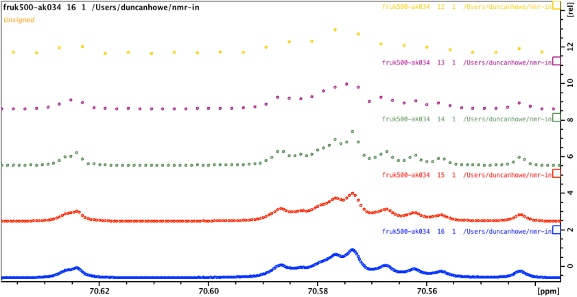
Zooming into the plot can show you some interesting things… This zoom shows that the temperature of the sample never quite reached perfect stability. This experiment ran a scan every 4 seconds and the temperature ramped up to the next one, 600 seconds after reaching +/- 0.1C stability.

The difference in temperature in the last 3 minutes is 0.154C, but there is still slight downwards trend and it looks as though equilibrium wouldn’t be reached for at least another 5 minutes.

So that was for the glycol sample at 500l per minute, how about at 800l per minute? Will the sample temperature be different? Will stability be reached at a faster rate? How about with a different reference sample and at different gas flows and chiller powers?

Here’s the results.

Well, beloware graphs of my findings… Each sample has its curve extrapolated past the temperature range it supposed to be valid for.

Well both the offset and the slope of the line can change; according to the sample and the conditions used.  Also over the regions that should overlap from the different reference samples; the values don’t match… So I’d say if you need *really* accurate temperature measurements from an experiment; run through the temperature calibrations carefully. Personally, I like the 99.8% CD3OD/0.2% CH3OH sample, as I think its less likely to be affected by radiation damping and the low viscosity should help it equilibrate faster.